Valentin De Bortoli, James Thornton, Jeremy Heng, Arnaud Doucet 
University of Oxford, UK
2021, Advances in Neural Information Processing Systems
[paper][blog][code]

•

이 포스트는 저자의 blog를 참고하여 작성되었습니다.

Intro & Overview

Overview

•

기존에는 Forward process를 사전 정의 후 Reverse process를 학습함.

•

DSB는 Forward process를 학습 가능하게 만듬.

•

핵심은 timestep t에서 Forward process에 해당하는 분포 P\mathbb{P}P와 Reverse process에 해당하는 분포 π⋆\pi^{\star}π⋆를 KL-divergence로 맞추어 주는 것.

Contribution

기존 Score-based moeling 방법과 달리 DSB의 수렴은 IPF의 수렴에 의해 결정

DSB 알고리즘은 기존 알고리즘 위에서 사용될 수 있음.
기존에 Score-based 모델에서 사용되었던 모든 기술이 DSB에 구현가능.

DSB는  ppriorp_{\text{prior}}pprior​가 가우시안일 필요가 없음. 
실제로 ppriorp_{\text{prior}}pprior​ 에서 샘플을 얻을 수 있기만 하면 됨. 
Gaussian이 아니라 다른 데이터셋이 될 수도 있음 (Dataset interpolation)

이로 인해 고차원의 최적 운송 (high-dimensional optimal transport)에 대한 Application이 기대됨.

Limitations

성능이 조금 떨어짐. 아키텍처 최적화가 덜 이루어짐.

아직 개선의 여지가 많음.

Preliminaries

Score-based generative modeling.

생성 모델링 (Generative Modeling)에서는 주어진 분포

p_{\mathrm{prior}}

를 주어진 데이터 분포

p_{\mathrm{data}}

로 변환 (Transform)하는 알고리즘을 설계하는데 관심이 있습니다. 데이터 분포

p_{\mathrm{data}}

는 샘플을 통해서만 접근할 수 있습니다.

최근 몇 년 동안, 생성 모델링은 기계 학습 및 이미지 처리에서 고전적인 작업이 되었습니다. 이 문제를 해결하기 위해 Energy-based Models, GANs, Normalizing Flow, VAE 또는 Diffusion Score-matching 과 같은 다양한 프레임워크가 연구되어왔습니다. Diffusion Model은 시각적 품질 측면에서 GAN을 능가하는 데 큰 가능성을 보여주었으며, 확산 과정의 이산화로 재구성 (discretization) 될 수 있으므로 수학적 관점에서도 매력적입니다.

점수 기반 생성 모델링의 기본 개념을 잠시 상기해 보겠습니다. 또한 Yang Song의 블로그 게시물에서 소개하거나 논문 [2,3]에서도 볼 수 있습니다.

다음과 같은 오른스타인-울렌베크 확산 (Ornstein-Ulhenbeck Diffusion)이 있습니다.

\mathrm{d} \mathbf{X}_t = -\alpha \mathbf{X}_t \mathrm{d} t + \sqrt{2} \mathrm{d} \mathbf{B}_t \ , \qquad \mathbf{X}_0 \sim p_{\mathrm{data}} \ , \alpha > 0.

Noising process

(\mathbf{X}_t)_{t \in [0,T]}

는 데이터 분포

p_{\mathrm{data}}

를 perturbing하는 과정입니다.

p_{\text{prior}}

를 이에 대한 불변분포 (invariant distribution)이라고 한다면, 다음과 같습니다.

p_{\mathrm{prior}} = \mathcal{N}(0,1/\alpha)

만약

T>0

이 충분히 크다면, 분포

\mathbf{X}_T

는

p_{prior}

에 가까워집니다. (OU process의 에르고딕 성질) 따라서 샘플링 과정은 다음과 같이 이루어집니다. 먼저

p_{\text{prior}}

로부터 샘플링하고,

(\mathbf{X}_t)_{t \in [0,T]}

의 Dynamics를 반전시켜 (Reversing)

p_{\text{data}}

를 샘플링합니다. 이러한 time-reversal operation은 놀랍게도 명시적인 (explicit) drift와 diffusion matrix를 가진 다른 디퓨전 프로세스로 연결됩니다. [4]

\mathrm{d} \mathbf{Y}_t = \{\alpha \mathbf{Y}_t + 2 \nabla \log p_{T-t}(\mathbf{Y}_{t}) \}\mathrm{d} t + \sqrt{2} \mathrm{d} \mathbf{B}_t \ , \qquad \mathbf{Y}_0 \sim p_{\mathrm{prior}} \ ,

여기서

p_t

는

\mathbf{X}_t

밀도입니다. 이전 디퓨전 프로세스에서 사용된 Euler-Maruyama 이산화를 적용하면 Markov chain 생성 모델을 얻을 수 있습니다.

Y_{k+1}^\star = Y_k^\star + \gamma_{k+1} \{\alpha Y_k^\star + 2 \nabla \log p_{T- t_k}(Y_k^\star)\} + \sqrt{2 \gamma_{k+1}} \ ,

with

\{\gamma_{k+1}\}_{k=0}^{N-1}

= sequence of stepsize,

t_k = \sum_{j=0}^{k-1} \gamma_{j+1}

하지만 이 Markov Chain

\{Y_k^\star\}_{k=0}^N

은 실제로 계산할 수 없는데, Stein-score

\nabla \log p_{t}

에 접근할 수 없기 때문입니다. 따라서 score-based generative modeling 에서는 이 점수는 다음 변분 문제 (variational problem)를 해결하는 신경망

s_{\theta^\star}

에 의해 근사됩니다.

\theta^\star = \mathrm{argmin}_\theta \mathrm{E}[\| \mathbf{Z}/\sigma_t + s_{\theta}(\mathbf{X}_t) \|^2] \ \,

여기서 오른스타인-울렌베크 프로세스의 해를 이용하면 다음과 같이 쓸 수 있습니다.

\mathbf{X}_t = m_t \mathbf{X}_0 + \sigma_t \mathbf{Z}

with

\mathbf{Z} \sim \mathcal{N}(0,1),\quad m_t=\exp[-\alpha t],\quad \sigma_t^2 = (1 - \exp[-2 \alpha t])/\alpha

s_{\theta^\star}

의 변분 공식 (Variational Formulation)은 다음과 같이 얻을 수 있습니다.

\nabla \log p_t (x) = \mathrm{E}[(m_t \mathbf{X}_0 - \mathbf{X}_t)/\sigma_t^2 | \mathbf{X}_t=x] = -\mathrm{E}[\mathbf{Z}/\sigma_t | \mathbf{X}_t=x]

따라서, 최종 Markov Process는 다음과 같습니다.

Y_{k+1} = Y_k + \gamma_{k+1} \{\alpha Y_k + 2 s_{\theta^\star}(T- t_k, Y_k)\} + \sqrt{2 \gamma_{k+1}} \ .

Generative model for CelebA. from Yang Song Blog.

점수 기반 생성 모델링의 주요 한계 중 하나는 초기 forward process가

p_{\text{prior}}

에 근접하도록 많은 양의 step를 요구하고 신경망 근사가 유지되도록 충분히 작은 크기의 stepsize를 요구한다는 것입니다.

이를 해결하기 위해 Diffusion Schrödinger Bridge가 제안되었습니다.

•

기존 Score-based Modeling의 일반화 버전.

•

Score-based 방법에 비해 필요한 stepsize의 수를 크게 줄일 수 있음.

•

ppriorp_{\text{prior}}pprior​가 Gaussian이어야 한다는 제한을 제거함

•

따라서 고차원 최적 운송 (Optimal Transport) 에 대한 가능성을 열음.

What is a Schrödinger Bridge?

슈뢰딩거 브릿지(SB, Schrödinger Bridge) 문제는 응용 수학, 최적 제어 및 확률에서 나타나는 classical problem입니다. [5, 6, 7]

이산-시간 (discrete-time setting)에서는 다음과 같은 동역학적 형태를 취합니다.

데이터에 노이즈를 추가하는 과정을 설명하는 분포

\mathbb{P}

의 Reference diffusion (

\mathbf{X}_t){t \in [0,T]}

우리의 목표는

\pi^\star_0 = p_{\text{data}}

와

\pi^\star_T = p_{\text{prior}}

인

\pi^\star

를 찾고,

\pi^\star

와

\mathbb{P}

의 KL-divergence를 최소화 하는 것입니다.

\pi^\star = \mathrm{argmin} \ \{\mathrm{KL}(\pi|\mathbb{P})\ , \ \pi_0 = p_{\mathrm{data}} \ , \ \pi_N = p_{\mathrm{prior}}\}

Diffusion Schrödinger Bridge (DSB)는 score-matching approaches를 사용하여 Iterative Proportional Fitting (IPF) 알고리즘을 근사합니다. IPF 알고리즘이란 SB 문제의 해답을 찾기위해 iterative (반복적인) 방법을 사용하는 알고리즘입니다.

DSB는 기존 SB의 개선된 버전으로 볼 수 있습니다. [5,6]

Discrete 세팅에서, IPF는 Sinkhorn algorithm이 됩니다. [8]

Methodology

Iterative Proportional Fitting (IPF) Algorithm

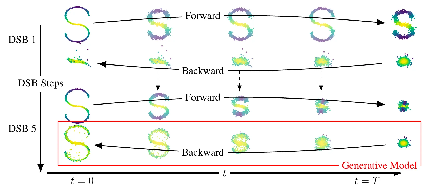
먼저 IPF를 알아보겠습니다. SB 문제의 해결책을 찾기 위해 IPF는 half-bridge problems를 연속적으로 해결함으로써 Iterative하게 작동합니다. 이렇게 해서, 우리는 distribution의 sequence

(\pi^n)_{n \in \mathbb{N}}

를 정의할 수 있습니다.

\pi^{2n+1} = \mathrm{argmin} \{ \mathrm{KL}(\pi|\pi^{2n}) \ , \ \pi_N = p_{\mathrm{prior}} \} \ , \\ \pi^{2n+2} = \mathrm{argmin} \{ \mathrm{KL}(\pi|\pi^{2n+1}) \ , \ \pi_0 = p_{\mathrm{data}} \} \ ,

with Initial condition

\pi^0 = \mathbb{P}

, (Reference Dynamics)

매우 큰

n

에 대해,

\pi^n

은 슈뢰딩거 브릿지

p^\star

에 가까워집니다.

따라서, 생성 모델은

\pi^{2n+1}

에서 샘플링하여 얻어집니다.

SB와 Score-based modeling의 관계

\pi^{2n}

이 다음 diffusion process의 측도 (measure)라고 가정합시다.

\pi^{2n}:\mathrm{d} \mathbf{X}_t^n = f_t^n(\mathbf{X}_t^n) \mathrm{d} t + \sqrt{2} \mathrm{d} \mathbf{B}_t \ , \quad \mathbf{X}_0^n \sim p_{\mathrm{data}} \ ,

그렇다면, time-reversal operation R에 대해

(\pi^{2n})^R

은 다음 diffusion process와 연관됩니다.

{(\pi^{2n})^R}:\mathrm{d} \mathbf{Y}_t^n = b_{T-t}^n(\mathbf{Y}_t^n) \mathrm{d} t + \sqrt{2} \mathrm{d} \mathbf{B}_t \ , \quad \mathbf{Y}_0^n \sim p_{\mathrm{prior}}

where

b_{t}^n(x) = -f_t^n(x) + 2 \nabla \log p_t^n(x) \ ,

with

p^n_t

is density of

\pi^{2n}_t

이 과정을 반복하면

\pi^{2n+2}

를 얻을 수 있습니다.

\pi^{2n+2}: \mathrm{d} \mathbf{X}_t^{n+1} = f_t^{n+1}(\mathbf{X}_t^{n+1}) \mathrm{d} t + \sqrt{2} \mathrm{d} \mathbf{B}_t \ , \quad \mathbf{X}_0^{n+1} \sim p_{\mathrm{data}} \ ,

where

f_{t}^{n+1}(x) = -b_t^n(x) + 2 \nabla \log q_t^n(x) \ ,

with

q^n_t

is density of

\pi^{2n+1}_t

이제 이 과정을 반복할 수 있습니다.

물론 위 역학에서 직접 샘플링할 수 없으며, Euler-Maruyama 근사를 사용하여 이산화합니다. 로그 그라디언트는 Score-matching 기술을 사용하여 근사됩니다. (그러나 메모리 문제로 인해 score가 아닌 drift 함수를 근사합니다). 이 이산화 및 변분 근사는 우리의 Diffusion Schrödinger Bridge알고리즘을 정의합니다.

몇 가지 장점:

기존 Score-based moeling 방법과 달리 DSB의 수렴은 IPF의 수렴에 의해 결정됩니다.

DSB 알고리즘은 기존 알고리즘 위에서 사용될 수 있습니다. 
따라서, 우리의 방법은 기존 Score-based 생성 모델의 개선 볼 수 있으며, 기존에 사용되었던 모든 기술이 DSB에 구현될 수 있습니다.

DSB는  ppriorp_{\text{prior}}pprior​가 가우시안일 필요가 없습니다. 실제로 ppriorp_{\text{prior}}pprior​ 에서 샘플을 얻을 수 있는 것만 필요합니다. 이는 다른 데이터셋일 수 있습니다. 이러한 성질을 이용해 dataset interpolation을 수행할 수 있습니다. 이는 고차원 최적 운송 (high-dimensional optimal transport)에 대한 추가적인 응용을 가능하게 합니다.

한계점:

DSB는 성능면에서 아직 조금 부족합니다. 점수 근사를 매개변수화 (parameterize)하기 위해 기존 아키텍처를 사용하기 때문에 계산 제한이 있습니다. 이 아키텍처는 깊고 불안정합니다 (예를 들어, EMA를 필요로 함)이는 DSB의 parameter를 신중하게 선택해야 함을 요구합니다.

Experimental Results

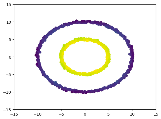
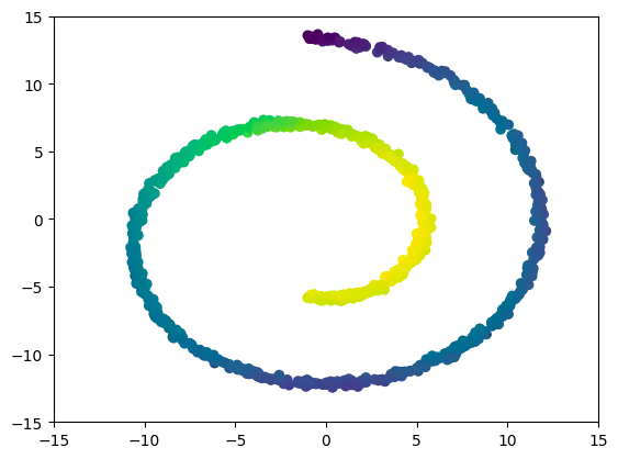
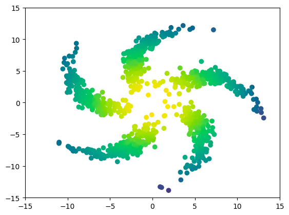
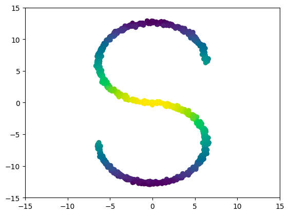
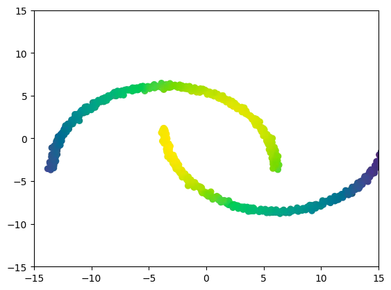
2차원 예시

MNIST

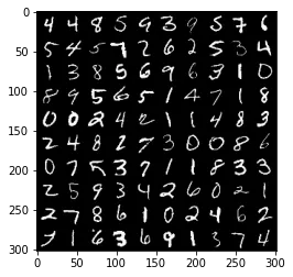
Original Dataset

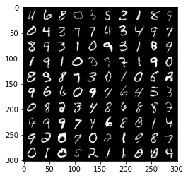
Generated Samples

DSB iterations에 따른 결과. 점점 퀄리티가 좋아짐.

CelebA

•

latent space exploration을 볼 수 있음

•

Gaussian random variables은 고정 → Deteministic.

•

latent space에서 Ornstein-Ulhenbeck process를 따르고 image space로의 deteministic mapping에 의한 transformation 을 볼 수 있음.

Dataset interpolation

•

두 Dataset간의 interpolation 시각화

References

[1] Prafulla Dhariwal and Alex Nichol Diffusion models beat GAN on Image Synthesis In: arxiv preprint:2105.05233

[2] Yang Song and Stefano Ermon Generative modeling by estimating gradients of the data distribution In: Advances in Neural Information Processing Systems 2019

[3] Jonathan Ho, Ajay Jain and Pieter Abbeel Denoising diffusion probabilistic models In: Advances in Neural Information Processing Systems 2020

[4] Hans Föllmer Random fields and diffusion processes In: École d'été de Probabilités de Saint-Flour 1985-1987

[5] Christian Léonard A survey of the Schrödinger problem and some of its connections with optimal transport In: Discrete & Continuous Dynamical Systems-A 2014

[6] Yongxin Chen, Tryphon Georgiou and Michele Pavon Optimal Transport in Systems and Control In: Annual Review of Control, Robotics, and Autonomous Systems 2020

[7] Aapo Hyvärinen and Peter Dayan Estimation of non-normalized statistical models by score matching In: Journal of Machine Learning Research 2005

[8] Gabriel Peyre and Marco Cuturi Computational Optimal Transport In: Foundations and Trends in Machine Learning 2019