EGSDE: Unpaired I2I Translation via Energy-Guided SDEs
Intro & Overview
•
이미지에서 domain-invariant / domain-specific feature를 정의하고 이를 이용해 energy function을 디자인했다.
•
그 결과 I2I, Multi domain transfer를 성공적으로 수행했다.
•
본인의 디자인을 PoE 개념으로 설명하거나 Classifier guidance는 제안하는 방법의 특별한 케이스라는 것을 설명하는 등 이론적 근거를 마련하는데 힘을 썼다.
•
다만 feature extractor의 선택이 너무 naive해서 아쉬웠다.
•
여러 측면으로 확장되기 좋은 연구라고 생각된다.
Prelimamaries
SBDMs
•
Forward Process.
를 의 unknown data distribution이라고 할 때, Forward Process 는 다음과 같다.
Drift coefficient 와 Diffusion coefficient 은 노이즈의 사이즈와 관련되고 perturbation kernel 를 결정한다.
•
Reverse Process
를 SDE의 marginal distribution이라고 할 때, 다음과 같이 정의된다.
•
Score-matching (SBDMs)
SBDMs 논문에서는 Score-matching을 적용해 score model 를 이용해 를 근사했다.
이를 SDE Solver로 풀면 되는데, SBDMs는 Euler-Maruyama solver를 사용해 이산화했다.
Unpaired Image to Image Translation
I2I Task는 다음과 같이 Formulation 할 수 있다.
Source Domain 과 Target Domain 이 Training Data로 주어졌을 때, Unpaired I2I의 목표는 Source domain의 이미지를 target domain의 이미지로 transfer하는 것이다. 이러한 과정은 이미지 에 conditioned된 target domain 상의 분포 을 디자인하는 것으로 formulation할 수 있다. 이때 결과 이미지는 다음 두 조건을 만족해야 한다.
•
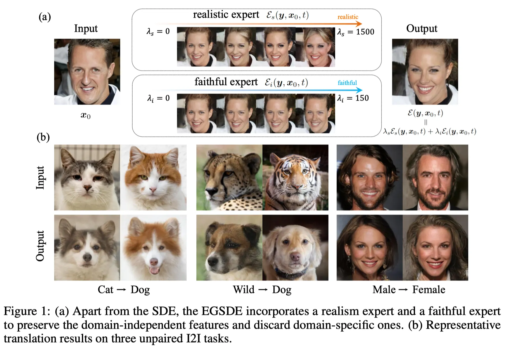
target domain 상에서 domain-specific features를 변화하며 realistic할 것.
•
source image 에 대해 domain-independent feature를 보존하며 faitful 할 것.
ILVR
ILVR은 target domain에 대해 diffusion model을 적용했다.
•
Realistic: 에서 시작해 (1)식으로 를 샘플링 함
•
Faithfulness: 샘플 와 perturbed source image 의 residual을 구하고 에 LPF ()를 이용해 더해줌.
SDEdit
•
Realistic: 에서 시작해 (1)식으로 를 샘플링 함
•
Faithfullness: Noisy Source image 로부터 샘플링을 함.
이때 는 structure를 잘 보존하는 숫자로 선택됨.
•
: marginal distribution conditioned on .
이러한 기존의 연구들은 training data의 source domain을 잘 활용하지 못했고 좋은 결과를 보여주지 못했다고 저자는 지적한다.
Methodology
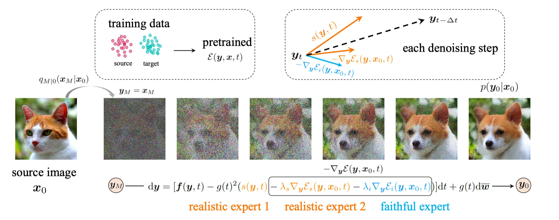
저자는 위에서 언급한 기존의 한계를 극복하기 위해 energy-guided SDEs를 제안한다.
•
두 도메인 상에 pre-trained된 에너지 함수를 이용해 inference process를 가이드한다.
•
먼저, 다음과 같이 pretrained SDE와 pretrained energy function을 사용해 을 정의한다.
1.
Score function 는 pretrained SDE이다.
2.
Energy function .
3.
Start point 은 perturbation distribution 으로부터 샘플링 되고 .
4.
이제 (2) 식을 이용해 최종 샘플을 얻을 수 있음.
여기서 SDE는 target domain에 의해서만 train되는건 똑같은데,
energy function이 target 과 source Domain 모두에 대해 train된 다는 것이 다르다고 주장한다.
그렇다면, 에너지 함수를 어떻게 잘 디자인해야 할까?
Choice of Energy
Cat → Dog 로 Translation하는 경우를 생각해보자. 이 경우, 다음과 같은 성질을 만족해야 한다.

1. Target Domain인 (Dog)로부터 domain-specific feature를 바꿈. (콧수염, 코 등)
2. Source Domain (Cat)으로부터 domain-independent feature을 보존함. (포즈, 컬러 등)
따라서, 에너지 함수를 다음과 같이 decompose 할 수 있다.
•
는 forward SDE로 구한 pertubed source image (Cat) 이다.
•
는 timestep 에서 까지의 perturbation kernel 이다.
•
은 log potential function이다.
•
은 와 sample간의 Similarity function이다.
•
위 디자인을 잘 보면, Source domain (e.g., Cat)은 Expectation을 통해 들어가고, target domain (Dog) 에 대한 정보는 score-function으로 직접 들어간다.
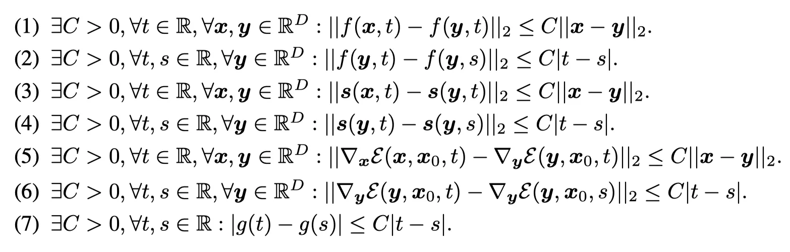
저자는 식 (4)에서 에 대한 기댓값 ()은 에너지 함수가 regularity condition을 만족하며 서서히 변화하는 것을 보장한다고 말한다.
좀 더 논의를 전개해보자.
먼저, 첫번째 아이디어를 만족하기 위한 디자인이다.
1. Target Domain인 (Dog)로부터 domain-specific feature를 바꿈. (콧수염, 코 등)
•
에서 time-dependent domain-specific feature extractor 을 도입한다.
•
는 Classifier가 된다. 왜냐하면..
◦
은 classifier에서 마지막 레이어를 제거한 것이다.
예를 들어 cat to dog의 경우, cat 혹은 dog를 분류하는 분류기가 된다.
◦
분류를 잘 하기 위해서는 domain-specific feature를 잘 보존하고 domain-independent feature를 날려버리게 된다.
•
은 generated sample과 source image들의 feature 간 cosine similarity로 정의된다.
•
는 spatial position 에서의 channel-wise feature가 된다.
•
식 (4)에 의해 domain-specific feature간의 cosine-similarity의 에너지 값은 최소화된다.
•
따라서 transffered sample은 domain-specific feature를 버리는 쪽으로 생성된다.
•
즉, 소스 이미지와 샘플의 같은 지점 에 대해 spatial 정보를 잘 보존한다.
•
classifier가 2-class 분류기 (cat, dog)라는 것이 target domain의 정보를 주입하는 핵심이다.
•
Training Time: domain-specific feature extractor for 5K iterations takes 7 hours based on 5 2080Ti GPUs.
여기서 조금 설득력이 부족하다고 생각했다.
domain specific feature를 classifier로 구한다는 건 좋은데, cos-sim를 최소화 한다는 것은 이를 Negative Pair로 간주하겠다는 것이다. 즉, 2-class classifier를 학습해서 사용하므로 “소스는 고양이니까, 무조건 반대로 가.” 라는 가이드밖에 못준다. 이건 “강아지” 쪽으로 가는게 아니라 “고양이”로부터 멀어질 뿐이다.
이 치명적인 한계는 논문에 언급되어있지 않다.
2. Source Domain인 Cat으로부터 domain-independent feature을 보존함. (포즈, 컬러 등)
•
에서 domain-independent feature extractor 을 도입한다.
•
는 LPF가 된다. 왜냐하면..
◦
domain-specific feature인 texture는 High-frequency 성분이고 domain-independent feature인 structure는 Low-frequency 성분이다.
◦
LPF는 domain-independent feature만을 남긴다.
◦
disentangled representation learning 연구에서 발전된 다른 방법도 있을 수 있으나, 명료하게 디자인의 효과를 보여주기 위해 가장 간단한 LPF를 선택했다.
•
은 generated sample과 source image의 LPF Feature간 negative squared distance이다.
•
식 (4)에 의해 domain-independent feature간의 L2 distance는 최소화된다.
•
따라서 transffered sample은 domain-independent eature를 보존하는 쪽으로 생성된다.
•
faithfulness: 즉, 소스 이미지와 샘플간의 domain-independent feature를 잘 보존하게 된다.
•
feature extractor 는 모두 guided diffusion에서 가져왔다.
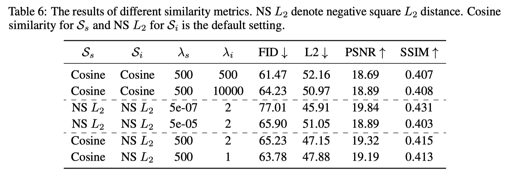
Similarity Metrics 의 선택
저자는 여러가지 metric에 대해서 실험을 해서 위와같이 디자인했다.
Energy Function의 디자인
또한, 초기 실험에서 식 (3) 대신 다음과 같은 간단한 Energy Function을 사용해보았다.
이것은 의 expectation이 필요없다. 하지만, noise-free 이미지와 노이즈가 존재하는 샘플간의 feature간의 similarity를 제대로 측정하지 않기 때문에 동작하지 않는다. (아래 표에서 Variant)
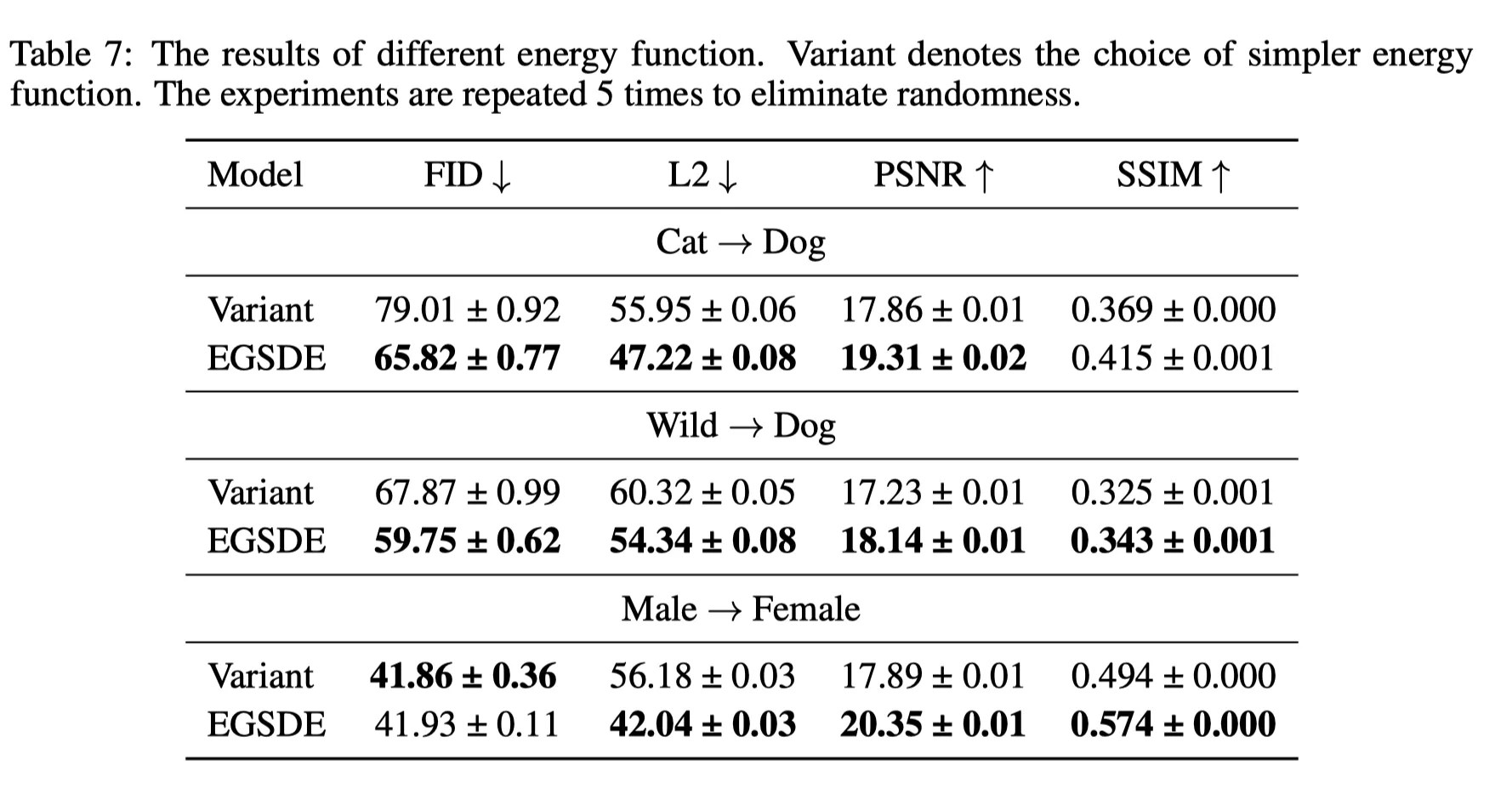
따라서 최종적으로 Design한 Energy function은 식 (3,4)와 같다.
Solving the Energy-guided reverse-time SDEs.
이제 pretrained score-based function 도 있고, Energy function 도 있다. 이제 conditional distribution 에서 샘플을 생성할 차례다.
먼저, conditional distribution은 다음 가정을 따른다. (Appendix A.1)
SBDMs의 Reverse-time SDEs의 해는 식 (1)과 같다.
EGSDE는 식(2)와 같다.
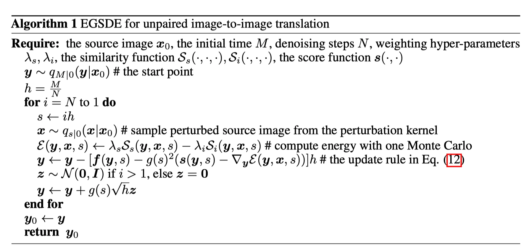
이제 SDE를 풀어보자. stepsize , iteration rule 은 에서 일때
•
Expectation 은 Monte Carlo를 single sample에 적용해 이용해 쉽게 구할 수 있다.
•
sample을 구하는 알고리즘은 다음과 같다.
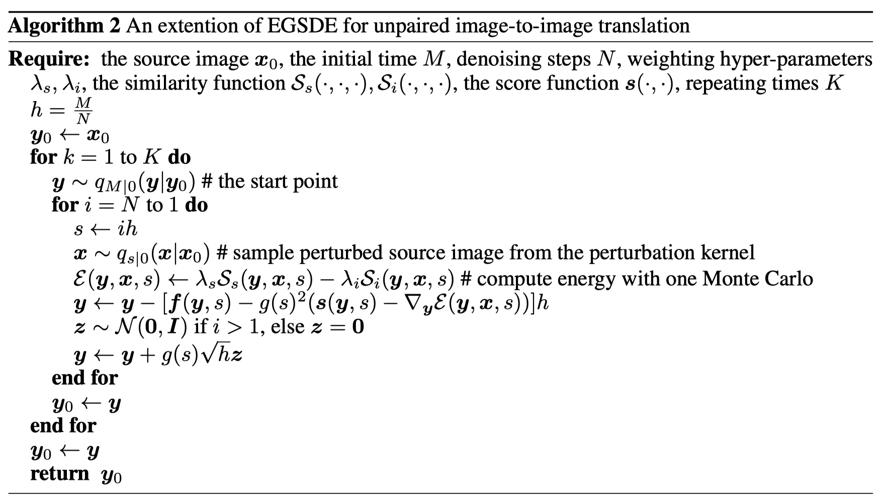
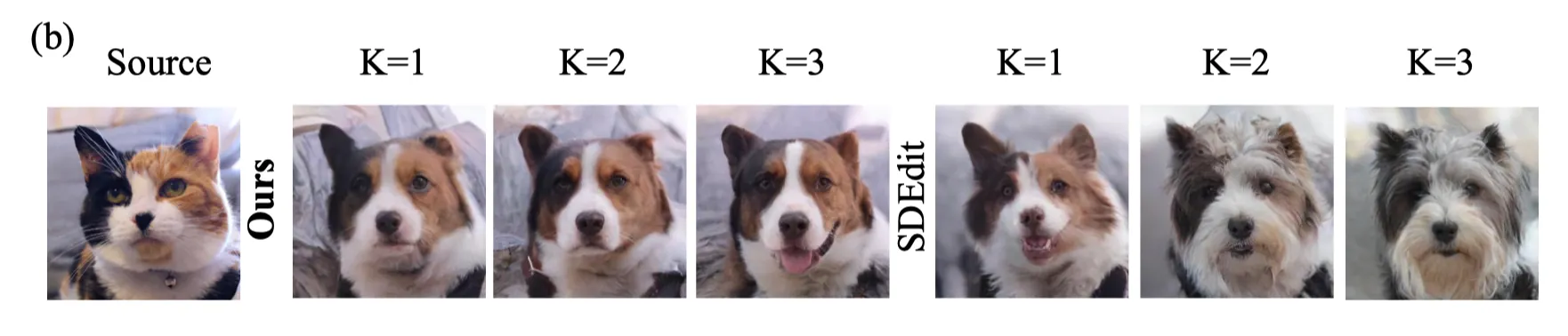
이 알고리즘을 K번 반복하면 다음과 같이 확장이 가능하다. (following SD-Edit , Appendix A.2)
•
DDPM의 Variance preserving을 사용하면 Noise Prediction Netwrok는 다음과 같이 된다.
•
Appendix A.3에 자세히 전개가 되어있다.
EGSDE 와 Classifier Guidance의 관계
에너지함수를 정의하는데 있어 pre-trained Classifier를 가져온 다는 것은 익숙한 접근이다. 그럼 classifier guidance와 어떤 관계가 있을까? 저자는 Appendix A.5에 이를 언급한다. 위 식(2)를 다시 가져오자.
이 식은 에 conditioned 되어 있는 분포 를 정의한다. time-dependent classifier 가 classifier이고 라고 하면, 다음과 같이 다시 쓸 수 있다.
이를 VP-EGSDE 식으로 풀면 classifier guidance와 같아진다.
저자는 Appendix 12에서 를 classifier guidance로 교체한 실험도 제공한다.
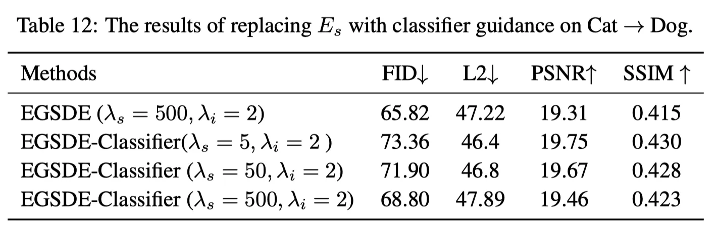
위 결과를 보면, Naive하게 Classifier를 적용한 것에 비해 더 좋은 결과를 얻은 것을 볼 수 있다.
EGSDE as Product of Experts
저자는 여기에 그치지 않고, Geofry Hinton의 Product of Expert (PoE)를 이용해 insight와 각 component의 role을 설명한다. (Appendix A.4)
•
conditional distribution 의 timestep 에 대한 PoE는 다음과 같다.
•
여기서 는 perturbation kernel이고, 와 은 time 에서의 marginal distribution이다. (SDEdit).
•
로부터 샘플하기 위해, transition kernel 를 정의하자. (.
•
•
는 partition function.
•
은 transition kernel이 된다.
◦
◦
•
가 에 대해 low curvature 를 가진다고 하면, Taylor Expansion으로 다음 식을 얻을 수 있다.
이 식을 보면, 식 (8)과 EGSDE의 discretization인 식 (6)의 같다는 것을 볼 수 있다.
따라서 에너지 유도 SDE를 이산화 방식으로 해결하는 것은 식 (7)의 PoE에서 샘플을 추출하는 것과 거의 동일하다. 식 (5)를 식 (7)에 대입하면 다음과 같이 된다.
이고, , 이다.
위 식 (10)에서 으로 하면 transffered sample은 3개의 expert에 의해 정의된 분포를 따른다.
•
realism expert : .
•
faithful expert: .
이런 PoE의 관점에서 EGSDE의 이론적 근거가 설명되었다고 저자는 말한다.
Experimental Results
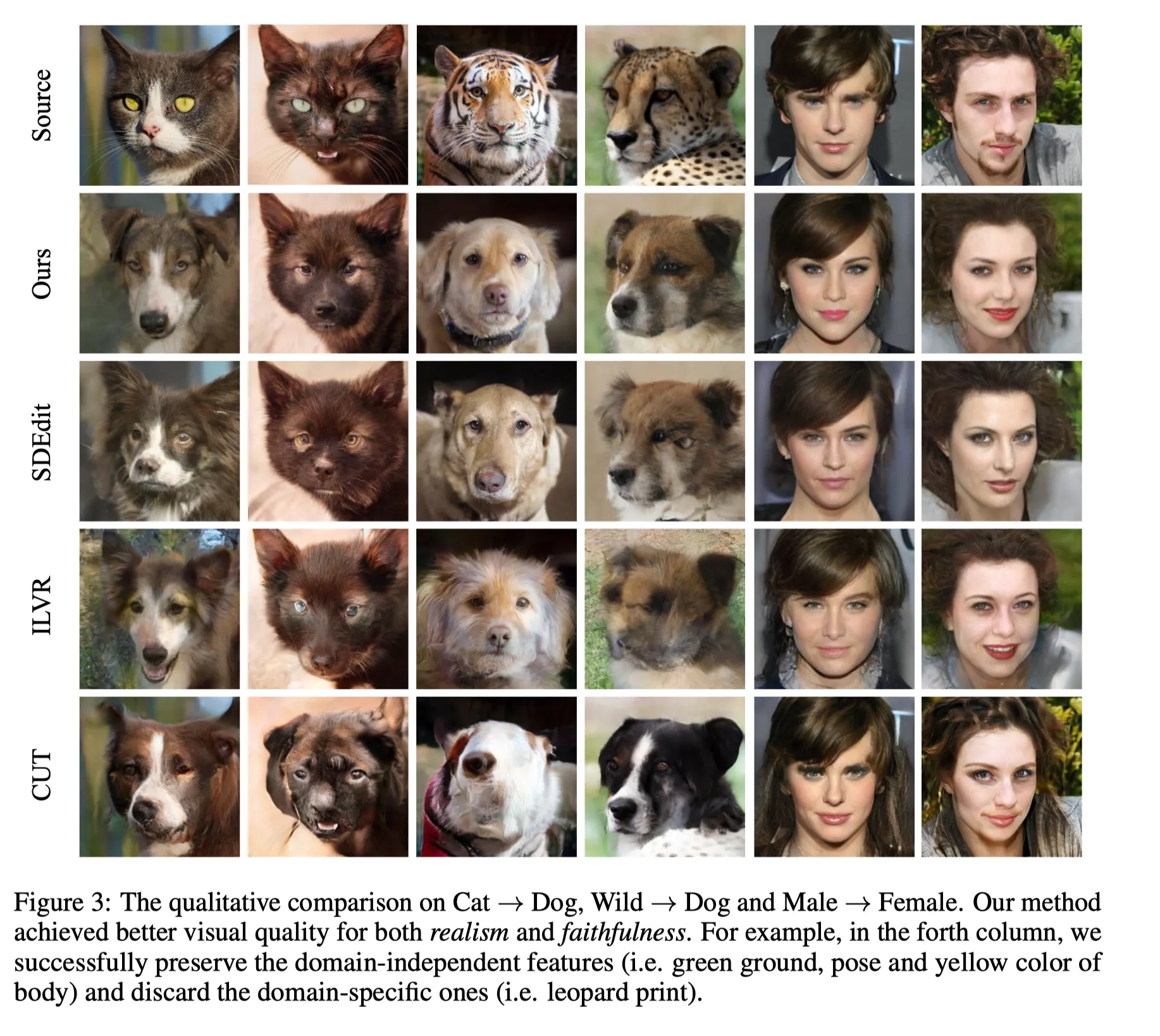
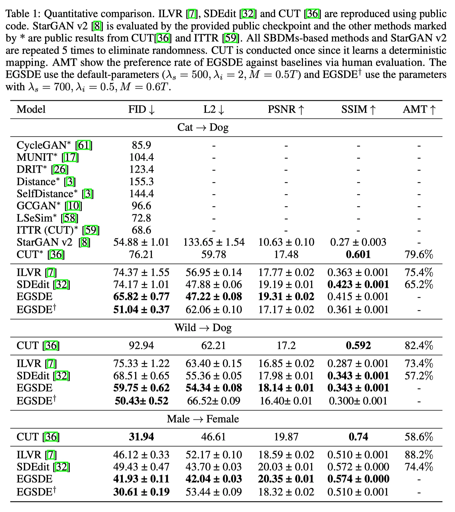
Two-Domain Unpaired Image Translation
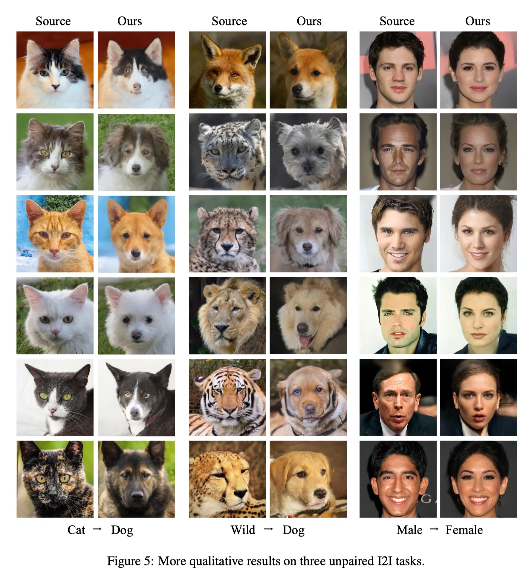
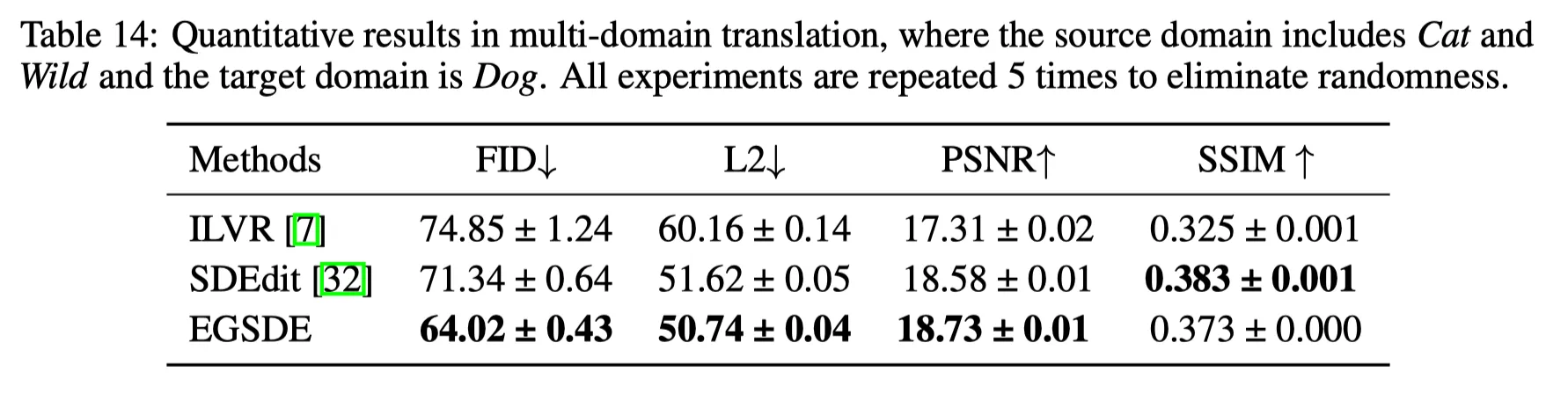
Multi-Domain Image Translation
의 translation이다.
차이점은, domain-specific feature extractor 이 3-class classifier라는 것이다.
실험 결과, 이 Task 역시 잘해낸다.
Ablation Studies
•
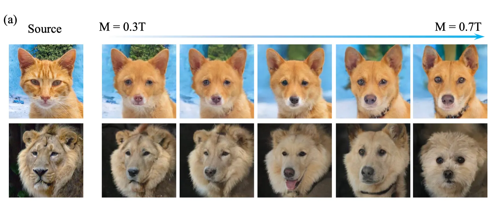
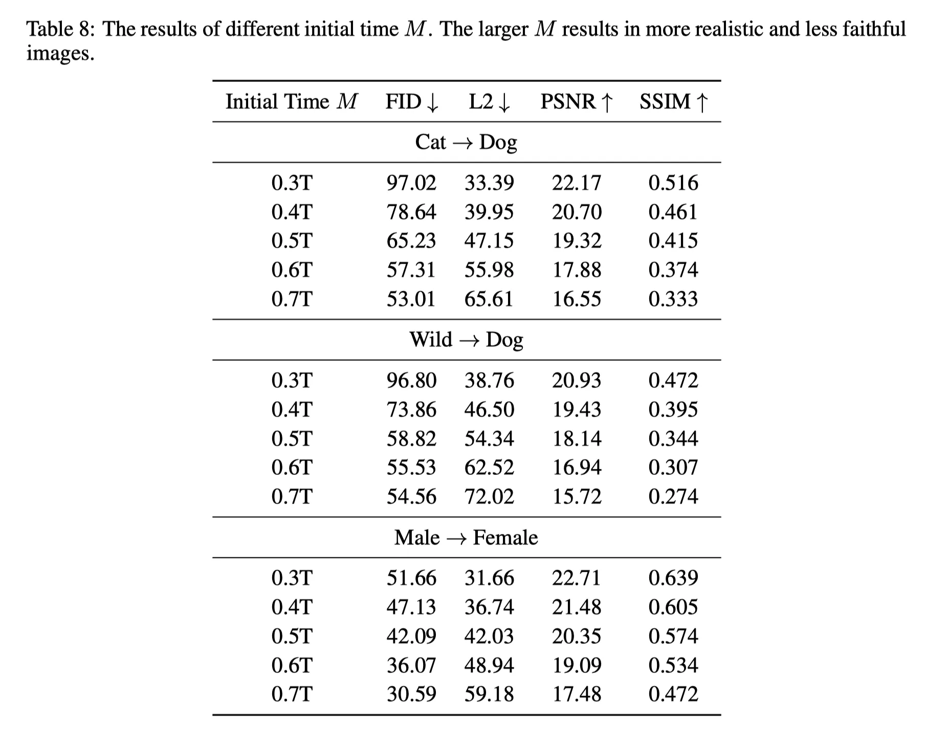
Initial Time M의 선택 (Figure 4, Table 8): 가 최적.
•
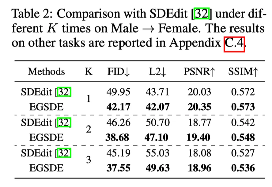
Repeating time 의 선택 (Figure 4, Table 2): K는 다다익선.
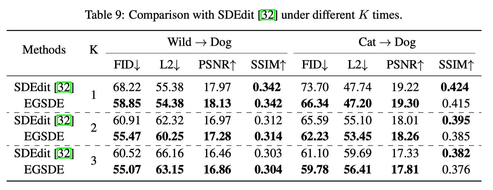
•
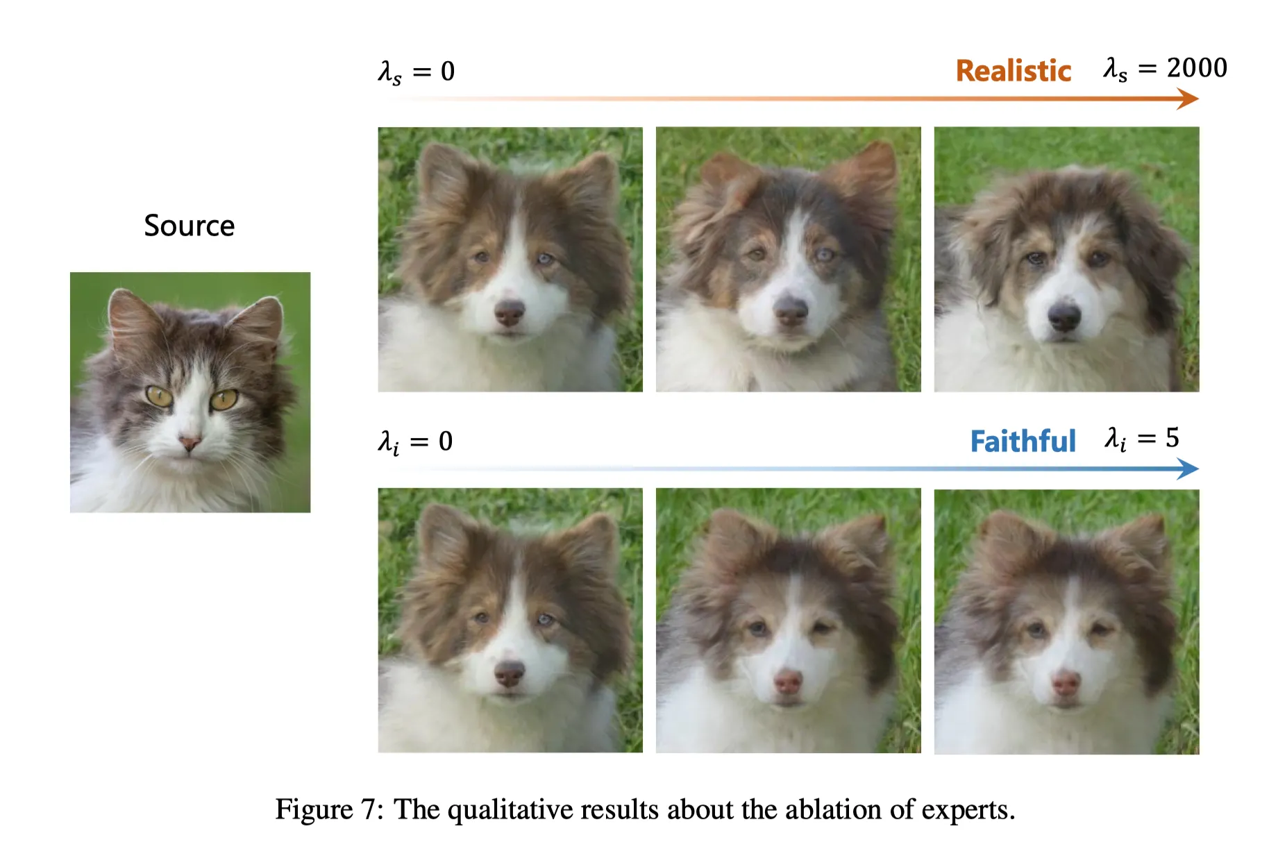
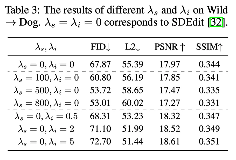
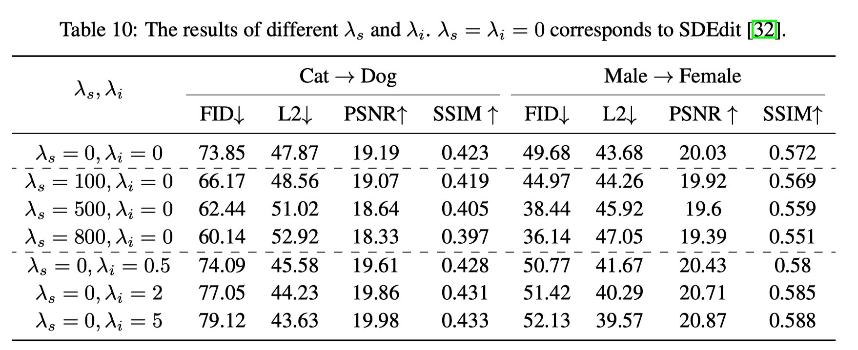
Expert function의 역할: 는 realistic image (FID↓), 는 faithful (L2↓)의 역할.
Conclusion
•
보통 Image Translation은 text 정보를 받아 CLIP 거리등으로 가이던스를 조절한다.
•
이 논문은, train과정에서 classifier의 분포를 학습하고 이를 이용해 image translation을 수행한다.
•
이 부분이 큰 한계점인데, 결국 one-to-one (많이 쳐줘도 Many-to-one)식의 translation만 가능할 뿐 아니라 각 도메인마다 train을 해주어야 한다는 것이다. 이런 단점은 논문에서 숨겨져 있다.
•
아무튼 저자는 효과적으로 domain-invariant feature와 domain-variant feature를 분리했다.
•
다만, feature extractor의 나이브한 선택이 아쉬웠다.
•
굳이 없어도 좋았을법 하지만 PoE를 도입해서 정당성을 설명하려 한 점이 인상적이었다.
•
sampling 측면이나 multi-domain 등으로 확장하기 좋은 연구라고 생각된다.
•
특히 text를 제거한 translation에 많은 insight를 줄 수 있다.