SDDM: Score-Decomposed Diffusion Models on Manifolds for Unpaired Image-to-Image Translation
Intro & Overview
Contribution of this work.
1.
Conditional Image Synthesis 중 얽힌 분포를 최적화하기 위해 SDDM을 개발, 이미지의 노이즈 제거 및 콘텐츠 세련 부분으로 점수 함수를 분해 (Decompose) 한다.
2.
SBDM의 조건부 생성에 다목적 최적화 알고리즘을 도입, 복잡한 gradient그라디언트 조합 알고리즘과 점수 인자 조정을 가능하게 하다.
3.
기존 저역 통과 필터보다 차원이 낮은 새로운 Block Adaptive Instance Normalization (BAdaIN) 모듈을 설계한다.
Controllable Generation with Score-based Model
•
•
score-based model에서 condtion은 다음과 같다.
•
Unpaired I2I를 해결하기 위해, EGSDE (Zhao et al., 2022) 는 두 개의 Energy-based guidance 함수를 설계했다.
하지만, 저자는 energy-based method가 중간 과정의 분포가 지나치게 또는 부정적으로 교란되는 것을 막을수 없었기 때문에, 둘 다 reference image의 statistics를 완전히 활용할 수 없었습니다. 그 결과 suboptimal한 결과가 나온다고 지적한다.
I2I Task에서의 기존 Score-based 모델의 한계
1.
Score guidance coefficient가 고정됨: 역 확산 과정의 확률 미분 방정식(SDE)으로 인해 Score-guidance의 coefficient가 고정되어 있어 모델 조정의 유연성이 제한된다.
2.
Energy Guidance 영향 불명확: 에너지 가이던스가 중간 분포에 미치는 영향이 명확하지 않아서 I2I Task에서 iteration이 충분하지 못할 때 결과가 불만족스러울 수 있다.
3.
중간 분포의 간섭: Guidance 과정 중 중간의 분포가 나쁜 영향의 간섭을 받지 않도록 보장하는 방법이 현재로서는 없다.
Proposed Method Overview
이를 극복하기 위해, 저자는 score function을 새로운 manifold 상에서 정의하고 분해 (decompose) 할 것을 제안합니다. 이를 통해 더욱 나은 에너지 가이던스와 statistical 가이던스를 제공할 수 있다고 주장한다.
Prelinamaries: Topology and manifolds
Basic Knowledge about Manifold.
집합 X가 주어졌을 때, 가 에 대해서 다음 세가지 조건을 만족하면 를 의 위상 (Topology) 라고 부르고, 를 위상공간 (Topological space)라고 부른다.
1.
2.
3.
이를 말로 풀어쓰면 다음과 같다.
1.
은 공집합과 전체집합을 포함한다.
2.
의 원소의 합집합은 에 속한다.
3.
의 원소의 유한 교집합은 에 속한다.
Definition 5. Topological space
A topological space is locally Euclidean of dimension if every point in has a neighborhood such that there is a homeomorphism from onto an open subset of . We call the pair ( ) a chart, a coordinate neighborhood or an open coordinate set, and a coordinate map or a coordinate system on . We say that a chart is centered at if . A chart about simply means that is a chart and .
정의 5: 위상 공간. 위상 공간에 대한 정의이다.
•
위상 공간 이 차원의 국소적으로 유클리드 공간이라는 것은 다음을 의미한다
◦
의 모든 점 가 그 점의 근방 를 가지고,
•
이러한 쌍 (을 차트라고 부른다.
•
이 차트 는 일때 를 중심으로 한다.
•
에 대한 차트 는 가 차트이고 라는 뜻이다.
Definition 6. Locally Euclidian property.
The locally Euclidean property means that for each , we can find the following:
•
an open set containing ;
•
an open set ; and
•
a homeomorphism (i.e., a continuous bijective map with continuous inverse).
정의 6. 국소적 유클리드 성질: 이는 의 각 점 에 대해, 를 포함하는 열린 집합 , 열린 집합 및 위상동형 (homeomorphism) 를 찾을 수 있다는 것을 의미한다.
즉, 의 모든 점 가 의 열린 집합과 위상동형인 네이버후드를 가진다는 뜻이다.
Definition 7. Topological manifold.
Suppose is a topological space. We say is a topological manifold of dimension or a topological -manifold if it has the following properties:
•
is a Hausdorff space: For every pair of points , there are disjoint open subsets such that and .
•
is second countable: There exists a countable basis for the topology of .
•
is locally Euclidean of dimension : Every point has a neighborhood that is homeomorphic to an open subset of .
1.
하우스도르프 공간이다.
2.
제 2 가산(최소한의 열린 집합 세트가 존재)이다
3.
국소적으로 차원 유클리드 공간과 동일하다.
Definition 8. Tangent vector.
A tangent vector at a point in a manifold is a derivation at .
정의 8. 접 벡터: 접 벡터는 다양체 의 점 에서의 미분이며, 이 점에서의 변화율을 나타낸다.
Definition 9. Tangent space.
As for , the tangent vectors at form a vector space , called the tangent space of at . We also write instead of .
정의 9. 접 공간: 에서와 마찬가지로, 에서의 접 벡터들은 벡터 공간 을 형성하며, 이는 의 에서의 접 공간이라고 불린다.
Definition 10. Normal space.
the normal space to at to be the subspace consisting of all vectors that are orthogonal to respect to the Euclidean dot product. The normal bundle of is the subset defined by with
정의 10. 정규 공간: 의 에서의 정규 공간은 유클리드 내적에 대해 와 직교하는 모든 벡터들을 포함하는 의 부분공간 으로 정의된다. 의 정규 번들은 에 정의된 의 부분집합 으로 정의된다.
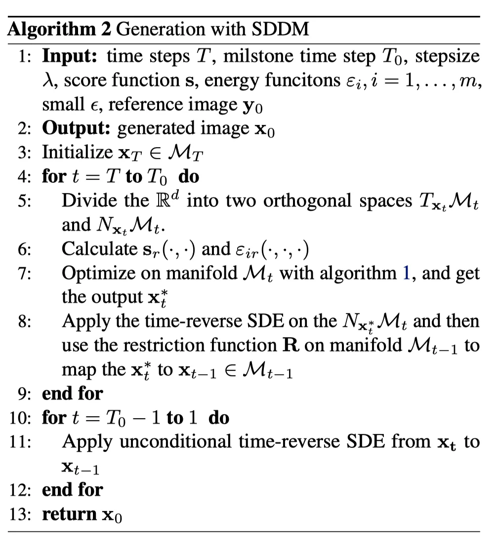
Methodology
저자는 위 EGSDE 의 모델로부터 논의를 시작한다. 위 모델에서 적절한 guidance function 를 선택해야 할 것입니다. 한편, 최신 연구 [Zhao et al. 2022, Bao et al. 2022b] 에서는 guidance function을 다음과 같은 형태를 사용한 것에 주목한다다.
이를 Score-Decomposed Diffusion Model이라고 한다.
그럼, Unpaired I2I를 위해서 어떻게 에너지 함수를 설계해야 할까?
Model Overview
To explicitly optimize the tangled distributions during image generation, we use moments of the perturbed reference image as constraints for constructing separable manifolds, thus disentangling the distributions of adjacent time steps.
•
timestep 와 에 대해, 두 매니폴드 와 는 separable.
•
따라서 conditional distribution 와 역시 separable.
•
이 때 매니폴드 는 score function 를 두 컴포넌트로 분해함.
◦
: content refinement part.
◦
: Denoising part.
•
마찬가지로 에서도 접공간 (tangent space) 평면 상에 존재하는 를 분해해 낼 수 있음.
•
따라서, optimization process는 다음과 같은 2단계로 이루어질 수 있음.
◦
1단계: Manifold 위에서 optimize.
▪
tangent space 상의 optimal direction인 MOO라는 빨간 벡터를 얻기 위해 알고리즘을 설계했다고 함.
◦
2단계: 다음 Manifold 로 적절하게 Mapping.
▪
이렇게 얻은 MOO 벡터를 위 식에 대입해 dx를 구하고, 를 다음 Manifold 로 mapping함.
▪
이때 는 consistency of form을 위한 Manifold 의 restriction이 됨.
언뜻 간단한데, 과연 어떻게 잘 동작하게될까?
이제 논문의 3.2는 수학적인 검증을 하게된다.
Decomposition of the Score and Energy Guidance
Score function이 다음과 같이 주어졌다고 해보자.
매니폴드 이 smooth, compact한 의 submanifold라고 가정하자. 그리고 은 이 매니폴드에 속한 (restriced) 확률분포이다. 그렇다면 다음과 같은 정의를 할 수 있다.
Definition 1. The tangent score function .
즉, 는 매니폴드 위에 존재한다. 만약 매니폴드 시리즈 와 원래 score function 가 있다면, 는 매니폴드 위의 tangent score function이다.
Definition 2. The tangent score function .
즉, 는 매니폴드의 normal space 위의 score function이다. 마찬가지로 는 매니폴드 위의 normal score function이다.
다음으로 다음과 같은 score function decomposition을 얻을 수 있다.
Lemma 1.
이는 를 알 때 파생될 수 있다.
일반적으로 이 Decomposition은 큰 의미가 없는데, 인접한 시간 단계들의 매니폴드들이 서로 결합되어 있기 때문이다. 이전 연구에서 전체 를 entire-manifold (Liu et al. 2022) 혹은 strong assumption (Chung et al. 2022) 으로 다루었다. 하지만, conditional generation task에서는 reference image 는 서로 다른 timestep에서 compact manifold를 제공할 수 있고 인접한 timestep의 manifold는 분리될 수 있다. 이런 관점에서 tangent score function은 매니폴드 상에서 refinement part로 간주될 수 있다. 그렇다면 normal score function은 매니폴드와 인접한 timestep간의 mappinf function이 된다.
따라서 manifold를 기술하는 proposition을 쓸 수 있다.
Proposition 1. At time step , for any single reference image , the perturbed distribution is concentrated on a compact manifold and the dimension of when is large enough. Suppose the distributions of perturbed reference image , where . The following statistical constraints define such .
이것을 풀어쓰자면, forward process로 얻어진 확률분포 은 콤팩트 매니폴드 상에 집중되고 매니폴드 의 차원은 보다 작다. 이므로, 에 대한 평균과 편차에 대한 제약이 매니폴드 를 정의한다는 것이다. 이렇게 정의된 매니폴드는 차원이므로 에 비해 차원이 적다. 이에 더해서, 차원을 더 낮추기 위해 ‘chunking trick’을 사용한다. 따라서 이러한 매니폴드를 사용하여 통계를 유지를 나타낼 수 있는데, 이는 tangnt space 이 "정제" 부분을 잘 분리 (separate) 할 수 있음을 나타낸다.
다음으로, 인접한 timestep에서의 와 또한 잘 분리될 수 있다는 Lemma 2를 기술한다.
Lemma 2. With the defined in Proposition 1, assume , Then and can be well separated. Rigorously, , divide the into two disconnect spaces where and .
한글로 풀어쓰자면 다음과 같다. 일 때 proposition 1에서 정의된 매니폴드 는 잘 분리될 수 있다. 엄밀하게 말해, 모든 에 대해, 를 두개의 연결되지 않은 공간 (disconnect spaces) 로 나누는 어떤 가 존재하고 이는 에 속한다. ( and .)
따라서, 를 사용해 score function 를 근사적으로 로 decompose할 수 있다. 좀 더 일반적으로 말해, 최적화공간 (optimization space)과 tangnt space 을 분리 (decouple) 할 수 있다. 를 이용해 SBDM의 score function과 energy 를 더 세밀하게 조작할 수 있다. 또한 “Refinement” 파트를 분리함으로써, score function의 “denoising” 파트가 지나치게 방해되는 것을 방지할 수 있다.
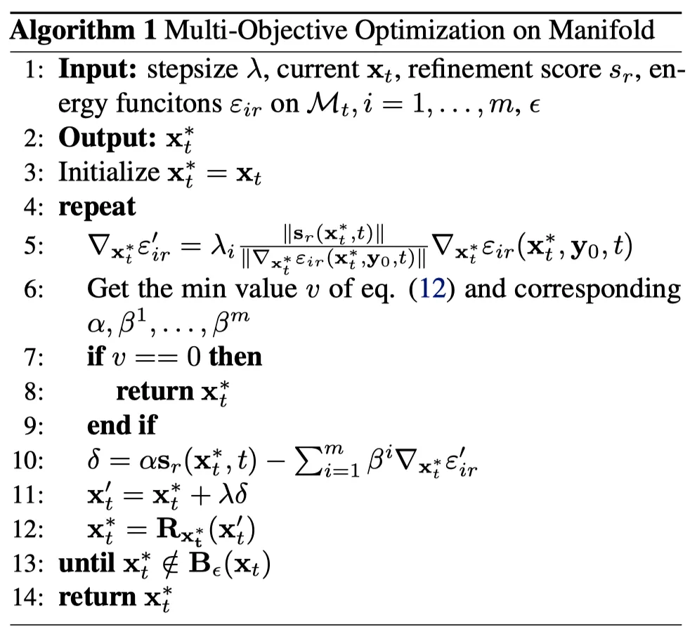
Stage 1: Optimization on Manifold.
Definition 3. Manifold Optimization.
Manifold optimization (Hu et al., 2020)은 실수 함수 를 주어진 리만 다양체 위에서 최적화하는 문제이다. Optimized target은 다음과 같다.
주어진 에 대한 score function 가 의 근사이므로 이제 를 의 potential energy가 된다. 그러므로 에너지 함수의 guidance가 된다.
Definition 4. Pareto optimality on the manifold.
라고 할 때,
•
만약 모든 에 대하여 이고 이면 는 를 지배(dominate) 한다.
•
만약 를 dominate하는 해 가 존재하지 않는다면, 그 해 는 파레토 최적이라고 불린다.
여기서 ‘지배’ (dominant)란 무엇일까? 이는 두 솔루션간의 비교평가에 대한 기술이다. 는 를 지배한다는 뜻은 해 가 objective에서 적어도 만큼 좋고 적어도 하나의 objective에 대해 분명하게 나은 경우를 말한다. 즉 에 비해 에서 더 나쁜 objective는 없으며, 적어도 하나의 objective에 대해서 더 낫다는 말이다. 이러한 를 찾지 못할 경우 는 파레토 최적인데, 이는 모든 objective에 대해 더 나은 솔루션이 없다는 뜻이다.
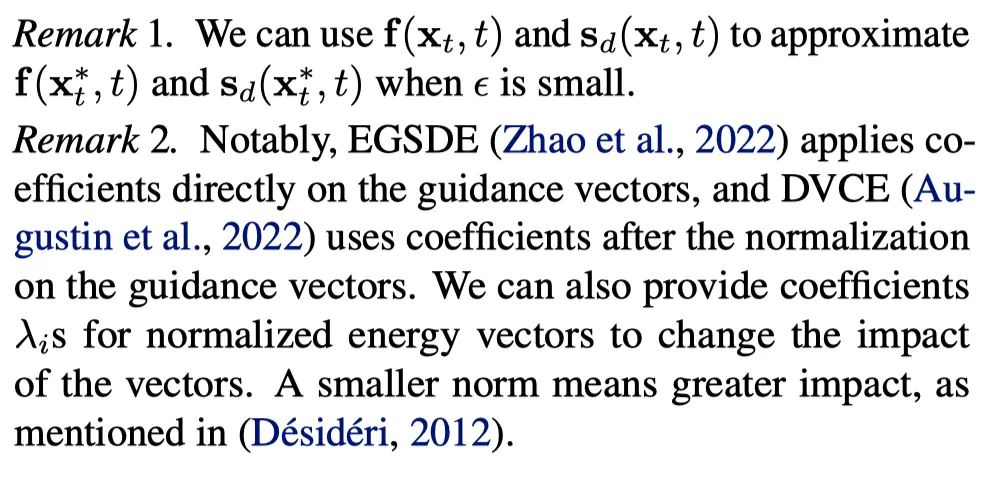
그렇다면, 다목적 최적화의 목표는 파레토 최적 해결책을 찾는 것이다. 지역 파레토 최적성은 단일 목적 최적화처럼 경사 하강법을 통해 달성될 수도 있다. 우리는 다중 경사 하강 알고리즘(MGDA) (Désidéri, 2012)을 따른다. MGDA는 또한 다목적 최적화를 위한 카루시-쿤-터커(KKT) 조건을 활용하는데, 이 방법에서는 다음과 같다.
Therom 1. K.K.T conditions on a smooth manifold.
At time step on the tangent space , there such that and , where are the fractions of on the tangent space and are functions restricted on the manifold .
이 Theorem 1은 특정 time step 에서의 매니폴드 접선공간 (tangent space)의 시나리오를 설명한다. 은 매니폴드 상에 제약되어있고, 은 의 접선공간 성분일때, 다음을 만족하는 가 존재한다.
•
•
위와 같은 조건을 만족하는 모든 점은 Parato stationary point라고 부른다. 모든 Pareto optimal point는 Pareto stationary point가 되고, 그 역은 성립하지 않는다. 이 문제의 해는 다음과 같다. (Desideri, 2012)
이를 통해 decent direction을 구할 수 있고 Pareto stationary point를 얻을 수 있다. 저자는 먼저 모든 gradient를 normalize했다.
Image to Image task에서, 많은 timestep에 대한 manifold 가 있으므로 작은 에 대해 Pareto stationary point를 에서 찾을 수 있다. 는 중심이 이고 지름이 인 open ball이다.
최종 알고리즘은 다음과 같다.
Stage 2. Transformation between adjacent manifolds.
manifold 에 대해 optimization을 했다면, 이제 를 dominate 하는 를 구했다. 이제 score function 의 “denoising” part , reverse-time noise와 rescriction function을 이용해 에서 로 mapping할 수 있다.
먼저, 인접 맵핑에 대한 성질을 다음 proposition으로 기술한다.
proposition 2. Suppose the is affine. Then the adjacent map has the following properties:
•
that
◦
정규공간 (Normal Manifold) 에 속하는 가 유일하게 존재하고, 와 더해지면 매니폴드 에 존재한다.
•
.
◦
매니폴드 에서 의 정규공간이 매니폴드 에서 의 정규공간과 동일하다.
•
is a transition map from to .
◦
는 매니폴드 의 접선공간 에서 매니폴드 의 접선공간 으로 이동하는 전이 맵이다.
•
is determined with , and .
◦
는 점 , 와 함수 에 의해 결정된다. 즉, 가 이런 입력에 의해 계산될 수 있다.
하지만, 를 adjecent map으로 사용하면 reverse-time noise와 의 영향을 잃게된다. 따라서 reverse SDE에 따라 normal space 상에 있는 추가 항과 상의 제한함수를 adjacent map으로 사용하는데, 이를 라고 표시한다.
이제 이미지를 생성하는 최종 알고리즘을 얻을 수 있다.